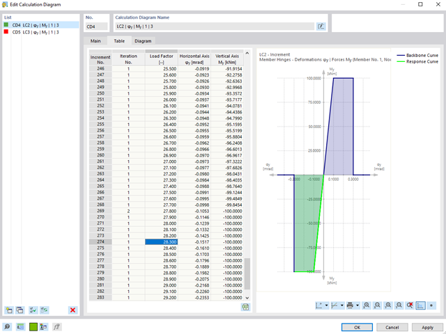
For calculation diagrams, the "2D | Hinge" is available. These hinge diagrams show the hinge response of load situations for nonlinear hinges.
For calculations with several load situations, such as is the case with pushover analyzes and time history analysis, you can evaluate the state of the hinge in each load step.
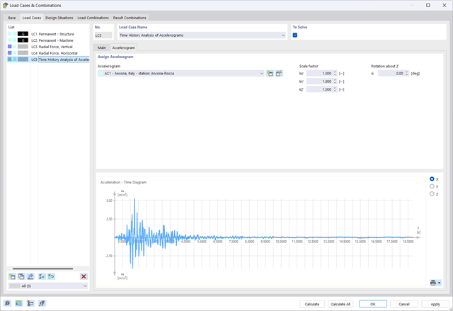
The Time History Analysis add-on provides you with accelerograms for the calculation. This extension allows for dynamic structural analysis of the acceleration-time diagrams.
There is an extensive library of earthquake records available for you, but you can also enter or import your own diagrams. The time history analysis is performed using the modal analysis or the linear implicit Newmark analysis.
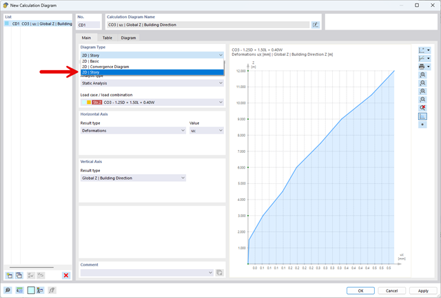
The "2D | Story" calculation diagram type is used to create result diagrams via the building axis. This allows you to easily analyze the behavior of the entire building under static and dynamic effects.
You can use this diagram type, for example, to visualize the seismic force over the building height.
- Analysis of time diagrams and accelerograms (acceleration-time diagrams exciting the supports of a structure)
- Combination of user-defined time diagrams with nodal, member, and surface loads, as well as free and generated loads
- Combination of several independent excitation functions
- Linear implicit Newmark analysis or modal analysis in time history
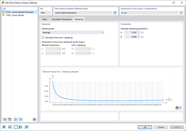
- Structural damping using Raleigh damping coefficients or Lehr's damping value
- Graphical display of results in calculation diagrams
- Result display in individual time steps or as an envelope during the entire time period
- Extensive library of seismic events (accelerograms)
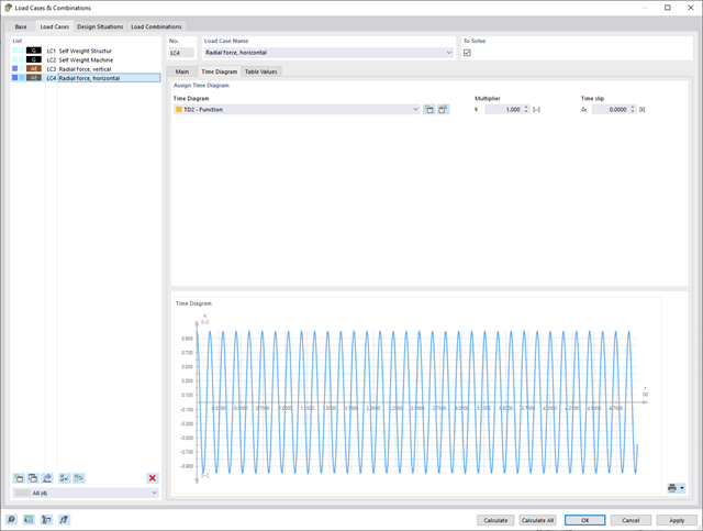
It is necessary to enter the required force-time diagrams. They can be combined in load cases or load combinations of the type Time History Analysis | Time Diagrams with the loading in order to define where and in which direction the force-time diagrams act.
The second option is to enter acceleration-time diagrams, which can be used in the load cases of the Time History Analysis | Accelerogram type.
All calculation parameters are specified in the time history analysis settings. These include, for example, the type of analysis method and the maximum calculation time.
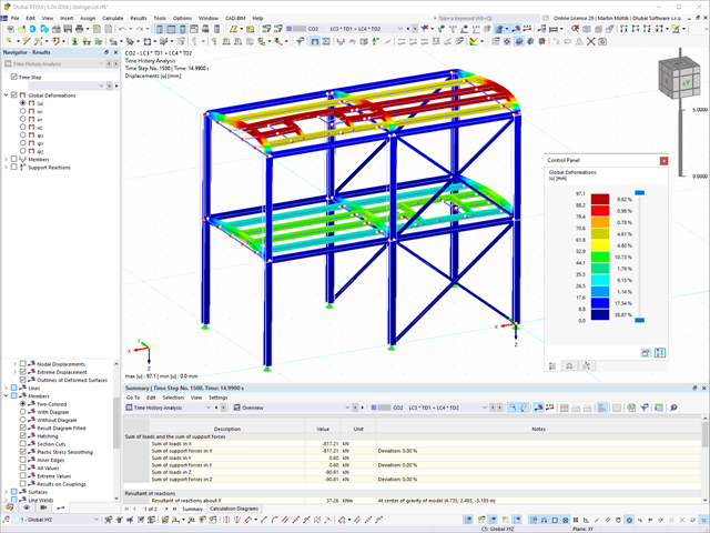
As soon as the program has completed the calculation, the summary of the results is listed. All result windows are integrated in the main program RFEM/RSTAB. You will find all the results arranged in tables; they can be displayed for each individual time step or as an envelope, and you also have the option of displaying the results graphically as well as animating them.
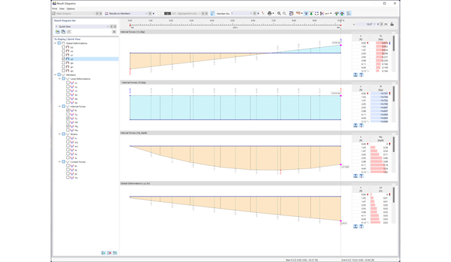
The results from the time history analysis can be displayed in the calculation diagrams. All the results are shown as a function of time. You can export the numeric values to MS Excel.
All result tables and graphics are part of the RFEM/RSTAB printout report. In this way, you can ensure clearly arranged documentation. You can also export the tables to MS Excel.
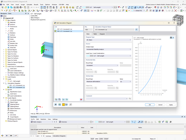
Do you want to create calculation diagrams? With RFEM and RSTAB, this works globally and without any problems. Create and organize your calculation diagrams directly in the Navigator - Data or via the menu Insert → Calculation Diagrams.
Use calculation diagrams to record and display a relation between the various calculation results.
It is also possible to superimpose similar diagrams.

Are you ready for the evaluation? Use the calculation diagrams, which show the distribution of a specific result during the calculation.
You can freely define the layout of the vertical and horizontal axes of the calculation diagram. This allows you, for example, to consider the settlement distribution of a certain node, depending on the load.
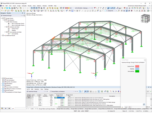
You can find the serviceability limit state design checks in the result tables of the Aluminum Design add-on. They are already fully integrated there. You have the option to display the design results with all the details at each location of the designed members. You can also use graphics with the result diagrams of the design ratios.
You can integrate all result tables and graphics into the global printout report of RFEM/RSTAB as a part of the aluminum design results. RFEM/RSTAB also allows you to display and document the deformations of the entire structure independently of the add-on.

RFEM allows you to use a special line hinge to model the special properties of the connection between the reinforced concrete slab and masonry wall. This limits the transferable forces of the connection depending on the specified geometry. You guess right: This means that the material cannot be overloaded.
The program develops interaction diagrams that are applied automatically. They represent the various geometric situations and you can use them to determine the correct stiffness.
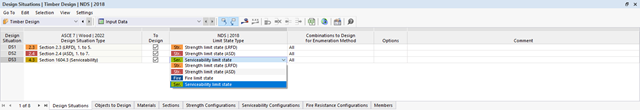
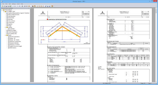
You find the serviceability limit state design fully integrated in the result tables of the Timber Design add-on. If yuo want to check the design results, you can open the program and display the results with all the details at each location of the designed members. Furthermore, graphics are available for you with the result diagrams of the design ratios.
A special thing is that All result tables and graphics can be integrated into the global printout report of RFEM/RSTAB as a part of the timber design results. You can also display and document the deformations of the entire structure as a part of the RFEM/RSTAB functionality. This function is independent of the add-on.
You can find the serviceability limit state design checks in the result tables of the Steel Design add-on. You can display the design results with all the details at each location of the designed members. Furthermore, graphics are available for you with the result diagrams of the design ratios. This gives you a good overview.
You can also integrate all result tables and graphics into the global printout report of RFEM/RSTAB as a part of the steel design results. Thus, you can display and document the deformations of the entire structure as a part of the RFEM/RSTAB functionality independent of the add-on.

Did you know that you can also display the moment-axial force interaction diagrams (M‑N diagrams) graphically? This allows you to display the cross-section resistance in the case of an interaction of a bending moment and an axial force. In addition to the interaction diagrams related to the cross-section axes (My‑N diagram and Mz‑N diagram), you can also generate an individual moment vector to create an Mres‑N interaction diagram. You can display the section plane of the M‑N diagrams in the 3D interaction diagram. The program displays the corresponding value pairs of the ultimate limit state in a table. The table is dynamically linked to the diagram so that the selected limit point is also displayed in the diagram.

- Calculation of stationary incompressible turbulent wind flow using the SimpleFOAM solver from the OpenFOAM® software package
- Numerical scheme according to the first and second order
- Turbulence models RAS k-ω and RAS k-ε
- Consideration of surface roughness depending on model zones
- Model design via VTP, STL, OBJ, and IFC files
- Operation via bidirectional interface of RFEM or RSTAB for importing model geometries with standard-based wind loads and exporting wind load cases with probe-based printout report tables
- Intuitive model changes via drag & drop and graphical adjustment assistance
- Generation of a shrink-wrap mesh envelope around the model geometry
- Consideration of environmental objects (buildings, terrain, and so on)
- Height-dependent description of the wind load (wind speed and turbulence intensity)
- Automatic meshing depending on a selected depth of detail
- Consideration of layer meshes near the model surfaces
- Parallelized calculation with optimal utilization of all processor cores of a computer
- Graphical output of the surface results on the model surfaces (surface pressure, Cp coefficients)
- Graphical output of the flow field and vector results (pressure field, velocity field, turbulence – k-ω field, and turbulence – k-ε field, velocity vectors) on Clipper/Slicer planes
- Display of 3D wind flow via animated streamline graphics
- Definition of point and line probes
- Multilingual user interface (German, English, Czech, Spanish, French, Italian, Polish, Portuguese, Russian, and Chinese)
- Calculations of several models in one batch process
- Generator for creating rotated models to simulate different wind directions
- Optional interruption and continuation of the calculation
- Individual color panel per result graphic
- Display of diagrams with separate output of results on both sides of a surface
- Output of the dimensionless wall distance y+ in the mesh inspector details for the simplified model mesh
- Determination of the shear stress on the model surface from the flow around the model
- Calculation with an alternative convergence criterion (you can select between the residual types pressure or flow resistance in the simulation parameters)
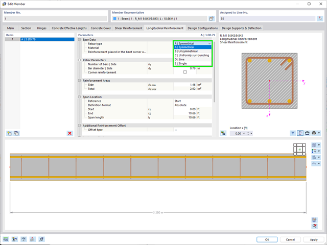
- Determination of longitudinal, shear, and torsional reinforcement
- Representation of minimum and compression reinforcement
- Determination of neutral axis depth, concrete and steel strains
- Design of member sections affected by bending about two axes
- Design of tapered members
- Design of RSECTION cross-sections (see this Product Feature)
- Determination of deformation in state II; for example, according to EN 1992‑1‑1, 7.4.3, and ACI 318‑19 24.2.3, Table 24.2.3.5
- Considering tension stiffening
- Considering creep and shrinkage
- Fatigue design according to EN 1992‑1‑1, Section 6.8 (see this Product Feature)
- Simplified fire resistance design according to EN 1992‑1‑2 for Columns (Section 5.3.2) and Beams (Section 5.6) (see this Product Feature)
- Seismic design according to EC 8 (see this Product Feature)
- Precise breakdown of reasons for failed design
- Design details of all design locations for better traceability of reinforcement determination
- Optional cross-section optimization
- Visualization of concrete section with reinforcement in 3D rendering
- Creation of 2D interaction diagrams; for example, M-N diagram
- Visualization of section resistance in 3D interaction diagram
- Output of moment-curvature diagram
Is the design completed? Then you can lean back. The design ratios of the individual design checks (for example, ultimate limit state, serviceability limit state, or compliance with the construction rules) are displayed for you in a table. You can also find the required reinforcement listed in clearly arranged output tables. The program shows you all intermediate values in a comprehensible manner.
You can display the results of members as result diagrams on the respective member. Furthermore, you have the option to document the inserted reinforcement for longitudinal and stirrup reinforcement, including sketches, in accordance with current practice.
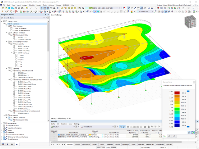
Select whether you want to display the results of surfaces as isolines, isosurfaces, or numerical values. In addition to the design check ratios, you can display the longitudinal reinforcement according to required, provided, and not covered reinforcement.

- Realistic representation of interaction between a building and soil
- Realistic representation of the influences of the foundation components on each other
- Extensible library of soil properties
- Consideration of several soil samples (probes) at different locations, even outside the building
- Determination of settlements and stress diagrams as well as their graphical and tabular display

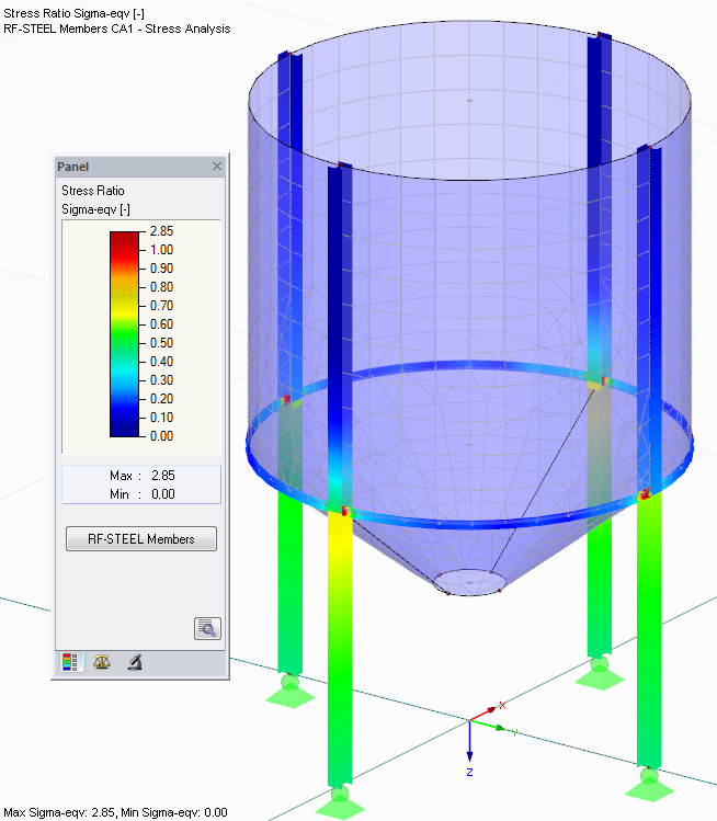
After you have completed the design, the program takes care of clearly arranged results. Thus, the program shows you the resulting maximum stresses and stress ratios sorted by section, member/surface, solid, member set, x-location, and so on. In addition to the tabular result values, the add-on shows you the corresponding cross-section graphic with stress points, stress diagram, and values as well. You can relate the design ratio to any kind of stress type. The current location is highlighted in the RFEM/RSTAB model.
In addition to the tabular evaluation, the program offers you even more. You can also graphically check the stresses and design ratios on the RFEM/RSTAB model. It is possible for you to adjust the colors and values individually.
The display of result diagrams of a member or set of members enables you a targeted evaluation. For each design location, you can open the respective dialog box to check the design-relevant section properties and stress components of any stress point. Finally, you have the option of printing the corresponding graphic, including all design details.
Customize the display of your data to your individual preferences. The result diagrams of members, surfaces (RFEM), and supports are freely configurable. You can define smooth ranges with average values or, if necessary, display and hide the result distributions. This ensures targeted evaluation of your results. Furthermore, you can easily add all diagrams to the printout report.
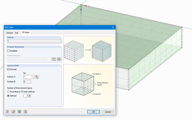
The stiffness of gas given by the ideal gas law pV = nRT can be considered in the nonlinear dynamic analysis.
The calculation of gas is available for accelerograms and time diagrams for both the explicit analysis and the nonlinear implicit Newmark analysis. To determine the gas behavior correctly, at least two FE layers for gas solids should be defined.
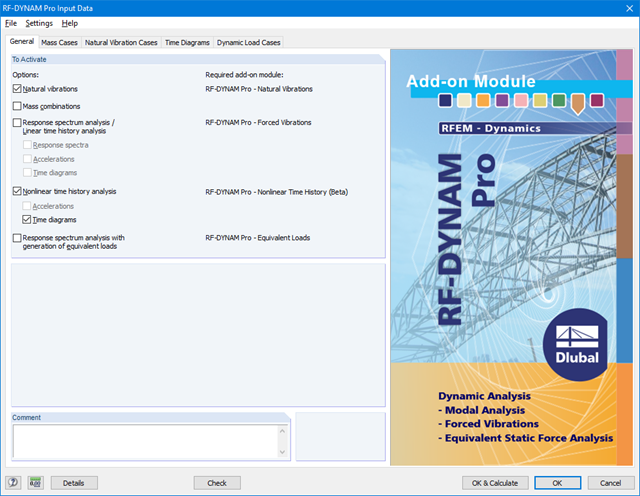
RF-/DYNAM Pro - Nonlinear Time History is integrated in the structure of RF‑/DYNAM Pro - Forced Vibrations and extended by two nonlinear analysis methods (one nonlinear analysis in RSTAB).
Force-time diagrams can be entered as transient, periodic, or as a function of time. Dynamic load cases combine the time diagrams with the static load cases, which provides high flexibility. Furthermore, it is possible to define time steps for the calculation, structural damping, and export options in the dynamic load cases.
.png?mw=640&hash=8cfd0c4bd093c03de543d147ffbf6f5c9250634a)
- User-defined time diagrams as a function of time, in tabular form, or as harmonic loads
- Combination of the time diagrams with RFEM/RSTAB load cases or combinations (enables definition of nodal, member, and surface loads, as well as free and generated loads varying over time)
- Combination of several independent excitation functions
- Nonlinear time history analysis with the implicit Newmark analysis (RFEM only) or the explicit analysis
- Structural damping using Rayleigh damping coefficients or Lehr's damping
- Direct import of initial deformations from a load case or combination (RFEM only)
- Stiffness modifications as initial conditions; for example, axial force effect, deactivated members (RSTAB only)
- Graphical display of results in a time history diagram
- Export of results in user-defined time steps or as an envelope
After the calculation, the maximum stresses and stress ratios are displayed sorted by sections, members/surfaces, member sets, or x-locations. In addition to the tabular result values, the corresponding cross-section graphic with stress points, stress diagram, and values is displayed as well. The design ratio can be related to any kind of stress type. The current location is highlighted in the RFEM/RSTAB model.
In addition to the result evaluation in the module, it is possible to represent the stresses and stress ratios graphically in the RFEM/RSTAB work window. It is possible to individually adjust the colors and values.
Result diagrams of a member or set of members facilitate targeted evaluation. Furthermore, you can open the respective dialog box of each design location to check the design-relevant section properties and stress components of any stress point. It is possible to print the corresponding graphic, including all design details.
- Import of materials, cross-sections, and internal forces from RFEM/RSTAB
- Steel design of thin‑walled cross‑sections according to EN 1993‑1‑1:2005 and EN 1993‑1‑5:2006
- Automatic classification of cross-sections according to EN 1993-1-1:2005 + AC:2009, Cl. 5.5.2, and EN 1993-1-5:2006, Cl. 4.4 (cross-section class 4), with optional determination of effective widths according to Annex E for stresses under fy
- Integration of parameters for the following National Annexes:
-
 DIN EN 1993-1-1/NA:2015-08 (Germany)
 -
 ÖNORM B 1993-1-1:2007-02 (Austria)
 -
 NBN EN 1993-1-1/ANB:2010-12 (Belgium)
 -
 BDS EN 1993-1-1/NA:2008 (Bulgaria)
 -
 DS/EN 1993-1-1 DK NA:2015 (Denmark)
 -
 SFS EN 1993-1-1/NA:2005 (Finland)
 -
 NF EN 1993-1-1/NA:2007-05 (France)
 -
 ELOT EN 1993-1-1 (Greece)
 -
 UNI EN 1993-1-1/NA:2008 (Italy)
 -
 LST EN 1993-1-1/NA:2009-04 (Lithuania)
 -
 UNI EN 1993-1-1/NA:2011-02 (Italy)
 -
 MS EN 1993-1-1/NA:2010 (Malaysia)
 -
 NEN EN 1993-1-1/NA:2011-12 (Netherlands)
 - NS EN 1993-1-1/NA:2008-02 (Norway)
-
 PN EN 1993-1-1/NA:2006-06 (Poland)
 -
 NP EN 1993-1-1/NA:2010-03 (Portugal)
 -
 SR EN 1993-1-1/NB:2008-04 (Romania)
 -
 SS EN 1993-1-1/NA:2011-04 (Sweden)
 -
 SS EN 1993-1-1/NA:2010 (Singapore)
 -
 STN EN 1993-1-1/NA:2007-12 (Slovakia)
 -
 SIST EN 1993-1-1/A101:2006-03 (Slovenia)
 -
 UNE EN 1993-1-1/NA:2013-02 (Spain)
 -
 CSN EN 1993-1-1/NA:2007-05 (Czech Republic)
 -
 BS EN 1993-1-1/NA:2008-12 (the United Kingdom)
 -
 CYS EN 1993-1-1/NA:2009-03 (Cyprus)
 - In addition to the National Annexes (NA) listed above, you can also define a specific NA, applying user‑defined limit values and parameters.
- Automatic calculation of all required factors for the design value of flexural buckling resistance Nb,Rd
- Automatic determination of the ideal elastic critical moment Mcr for each member or set of members on every x-location according to the Eigenvalue Method or by comparing moment diagrams. You only have to define the lateral intermediate supports.
- Design of tapered members, unsymmetric sections or sets of members according to the General Method as described in EN 1993-1-1, Cl. 6.3.4
- In the case of the General Method according to Cl. 6.3.4, optional application of "European lateral-torsional buckling curve" according to Naumes, Strohmann, Ungermann, Sedlacek (Stahlbau 77 [2008], pp. 748‑761)
- Rotational restraints can be taken into account (trapezoidal sheeting and purlins)
- Optional consideration of shear panels (for example, trapezoidal sheeting and bracing)
- RF-/STEEL Warping Torsion module extension (license required) for stability analysis according to the second-order analysis as stress analysis including consideration of the 7th degree of freedom (warping)
- Module extension RF-/STEEL Plasticity (license required) for plastic analysis of cross‑sections according to Partial Internal Forces Method (PIFM) and Simplex Method for general cross‑sections (in connection with the RF‑/STEEL Warping Torsion module extension, it is possible to perform the plastic design according to the second‑order analysis)
- Module extension RF-/STEEL Cold-Formed Sections (license required) for ultimate and serviceability limit state designs for cold-formed steel members according to the EN 1993-1-3 and EN 1993-1-5 standards
- ULS design: Selection of fundamental or accidental design situations for each load case, load combination, or result combination
- SLS design: Selection of characteristic, frequent, or quasi-permanent design situations for each load case, load combination, or result combination
- Tension analysis with definable net cross-section areas for member start and end
- Weld designs of welded cross-sections
- Optional calculation of warp spring for nodal support on sets of members
- Graphic of design ratios on cross-section and in RFEM/RSTAB model
- Determination of governing internal forces
- Filter options for graphical results in RFEM/RSTAB
- Representation of design ratios and cross‑section classes in the rendered view
- Color scales in result windows
- Automatic cross-section optimization
- Transfer of optimized cross-sections to RFEM/RSTAB
- Parts lists and quantity surveying
- Direct data export to MS Excel
- Verifiable printout report
- Possibility to include the temperature curve in the report
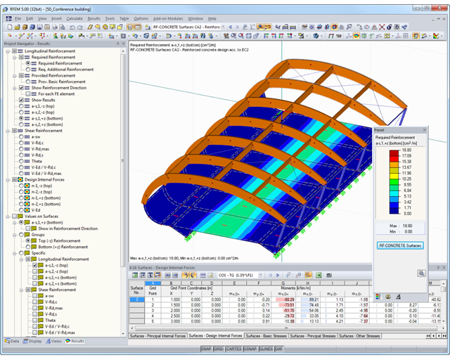
RF-CONCRETE Surfaces
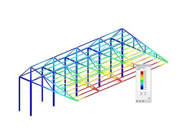
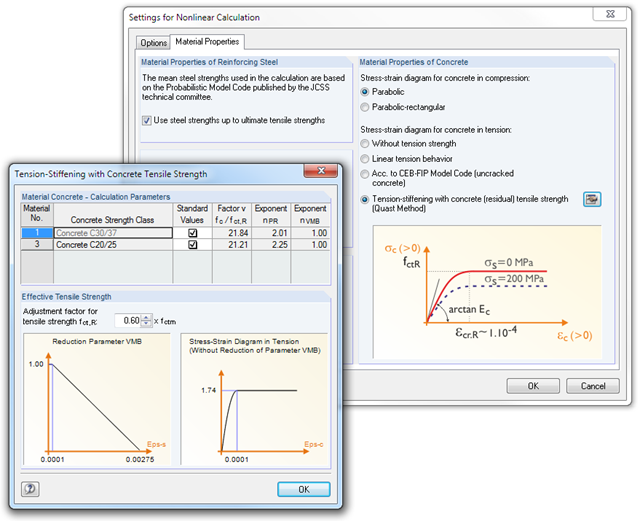
The nonlinear calculation is activated by selecting the design method of the serviceability limit state. You can individually select the analyses to be performed as well as the stress-strain diagrams for concrete and reinforcing steel. The iteration process can be influenced by these control parameters: convergence accuracy, maximum number of iterations, arrangement of layers over cross-section depth, and damping factor.
You can set the limit values in the serviceability limit state individually for each surface or surface group. Allowable limit values are defined by the maximum deformation, the maximum stresses, or the maximum crack widths. The definition of the maximum deformation requires additional specification as to whether the non-deformed or the deformed system should be used for the design.
RF-CONCRETE Members
The nonlinear calculation can be applied to the ultimate and the serviceability limit state designs. In addition, you can specify the concrete tensile strength or the tension stiffening between the cracks. The iteration process can be influenced by these control parameters: convergence accuracy, maximum number of iterations, and damping factor.
The following material models are available in RF − MAT NL:
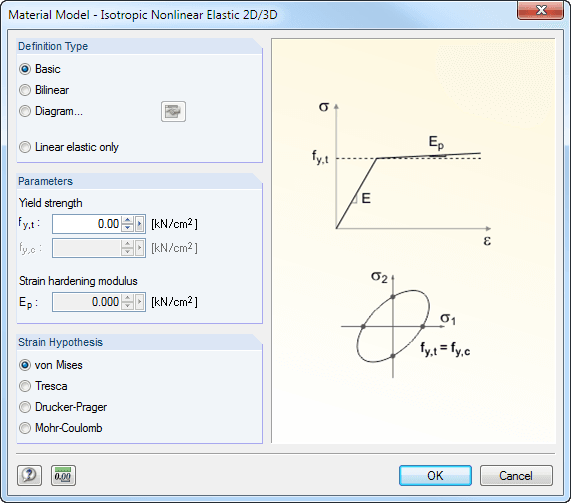
Isotropic Plastic 1D/2D/3D and Isotropic Nonlinear Elastic 1D/2D/3D
You can select three different definition types here:
- Basic (definition of the equivalent stress under which the material plastifies)
- Bilinear (definition of the equivalent stress and strain hardening modulus)
- Diagram:
- Definition of polygonal stress-strain diagram
- Option to save / import the diagram
- Interface with MS Excel
Orthotropic Plastic 2D/3D (Tsai-Wu 2D/3D)
This material model allows the definition of material properties (modulus of elasticity, shear modulus, Poisson's ratio) and ultimate strengths (tension, compression, shear) in two or three axes.
Isotropic Masonry 2D
It is possible to specify the limit tension stresses σx,limit and σy,limit as well as the hardening factor CH.
Orthotropic Masonry 2D
The material model Orthotropic Masonry 2D is an elastoplastic model that additionally allows softening of the material, which can be different in the local x- and y-directions of a surface. The material model is suitable for (unreinforced) masonry walls with in-plane loads.
Isotropic Damage 2D/3D
Here, you can define antimetric stress-strain diagrams. The modulus of elasticity is calculated in each step of the stress-strain diagram using Ei = (σi -σi-1 )/(εi -εi-1 ).
- Import of results from RSTAB
- Integrated material and cross-section library
- The module extension EC2 for RSTAB enables design of reinforced concrete according to EN 1992-1-1 (Eurocode 2) and the following National Annexes:
-
DIN EN 1992-1-1/NA/A1:2015-12 (Germany)
-
ÖNORM B 1992-1-1:2018-01 (Austria)
-
Belgium NBN EN 1992-1-1 ANB:2010 for design at normal temperature, and NBN EN 1992-1-2 ANB:2010 for fire resistance design (Belgium)
-
BDS EN 1992-1-1:2005/NA:2011 (Bulgaria)
-
EN 1992-1-1 DK NA:2013 (Denmark)
-
NF EN 1992-1-1/NA:2016-03 (France)
-
SFS EN 1992-1-1/NA:2007-10 (Finland)
-
UNI EN 1992-1-1/NA:2007-07 (Italy)
-
 LVS EN 1992-1-1:2005/NA:2014 (Latvia)
 -
LST EN 1992-1-1:2005/NA:2011 (Lithuania)
-
MS EN 1992-1-1:2010 (Malaysia)
-
NEN-EN 1992-1-1+C2:2011/NB:2016 (Netherlands)
- NS EN 1992-1 -1:2004-NA:2008 (Norway)
-
PN EN 1992-1-1/NA:2010 (Poland)
-
NP EN 1992-1-1/NA:2010-02 (Portugal)
-
SR EN 1992-1-1:2004/NA:2008 (Romania)
-
SS EN 1992-1-1/NA:2008 (Sweden)
-
SS EN 1992-1-1/NA:2008-06 (Singapore)
-
STN EN 1992-1-1/NA:2008-06 (Slovakia)
-
SIST EN 1992-1-1:2005/A101:2006 (Slovenia)
-
UNE EN 1992-1-1/NA:2013 (Spain)
-
CSN EN 1992-1-1/NA:2016-05 (Czech Republic)
-
BS EN 1992-1-1:2004/NA:2005 (United Kingdom)
-
 CPM 1992-1-1:2009 (Belarus)
 -
CYS EN 1992-1-1:2004/NA:2009 (Cyprus)
-
- In addition to the National Annexes (NA) listed above, you can also define a specific NA, applying user‑defined limit values and parameters.
- Optional presetting of partial safety factors, reduction factors, neutral axis depth limitation, material properties, and concrete cover
- Determination of longitudinal, shear, and torsional reinforcement
- Design of tapered members
- Cross‑section optimization
- Representation of minimum and compression reinforcement
- Determination of editable reinforcement proposal
- Crack width analysis with optional increase of the required reinforcement in order to keep the defined limit values of the crack width analysis
- Nonlinear calculation with consideration of cracked cross‑sections (for EN 1992‑1‑1:2004 and DIN 1045‑1:2008)
- Considering tension stiffening
- Considering creep and shrinkage
- Deformations in cracked sections (state II)
- Graphical representation of all result diagrams
- Fire resistance design according to the simplified method (zone method) according to EN 1992‑1‑2 for rectangular and circular cross‑sections. Thus, fire resistance design of brackets is possible as well.
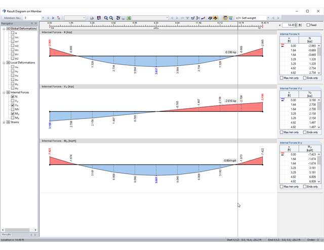
After the calculation, the results of performed designs, including all required intermediate values, are displayed in clearly arranged result tables sorted by various criteria. Since the program displays the intermediate values in detail, the transparency of all designs is ensured. It is possible to display the distribution of internal forces for each x-location of the beam in a separate graphical window. Here, both the deformations and the individual internal forces can be displayed.
Designs with design details and selected result diagrams can be added in the printout report, providing clearly arranged documentation. The printout report can include graphics, descriptions, drawings, and more. Moreover, it is possible to select which calculation data will be covered in the printout.
After the calculation, the module displays results in clearly arranged result tables. All intermediate values (for example, governing internal forces, adjustment factors, and so on) can be included in order to make the design more transparent. The results are listed by load case, cross-section, member, and set of members.
If the analysis fails, the relevant cross-sections can be modified in an optimization process. It is also possible to transfer the optimized cross-sections to RFEM/RSTAB to perform a new calculation.
The design ratio is represented with different colors in the RFEM/RSTAB model. This way, you can quickly recognize critical or oversized areas of the cross-section. Furthermore, result diagrams displayed on the member or set of members ensure targeted evaluation.
In addition to the input and result data, including design details displayed in tables, you can add all graphics into the printout report. This way, comprehensible and clearly arranged documentation is guaranteed. You can select the report contents and extent specifically for the individual designs.
The result diagrams of members, surfaces, and supports are freely configurable: You can define smooth ranges with average values or, if necessary, display and hide the result diagrams. This option ensures targeted evaluation of the results. All diagrams can be added in the printout report.